Online Alternatives Testing Pt 2 : l0stinsp4ce

Online Alternative Testing (part II)

An Implementation

Building off the last post, here's an iPython-notebook-ready implementation:

import numpy as np
import pandas as pd
import seaborn as sns
from scipy.stats import beta, uniform
TRUE_CTR = [.02, .012, .03]
# initialize priors as if we'd seen 3 clicks and 100 impressions
CTR_DISTS = [beta(3, 97)] * len(TRUE_CTR)  
UNIFORM = uniform(0, 1)
LOGS = []

def is_clicked(cta_idx):
    return UNIFORM.rvs(1) < TRUE_CTR[cta_idx]

def draw_cta_index():
    draws = np.hstack([dist.rvs(1) for dist in CTR_DISTS])
    return draws.argmax()

def update_dist(outcome, dist):
    alpha_param, beta_param = dist.args
    if outcome:
        alpha_param += 1
    else:
        beta_param += 1
    return beta(alpha_param, beta_param)

def step():
    cta_idx = draw_cta_index()
    outcome = is_clicked(cta_idx)
    CTR_DISTS[cta_idx] = update_dist(outcome, CTR_DISTS[cta_idx])
    LOGS.append((cta_idx, outcome))

Some results:

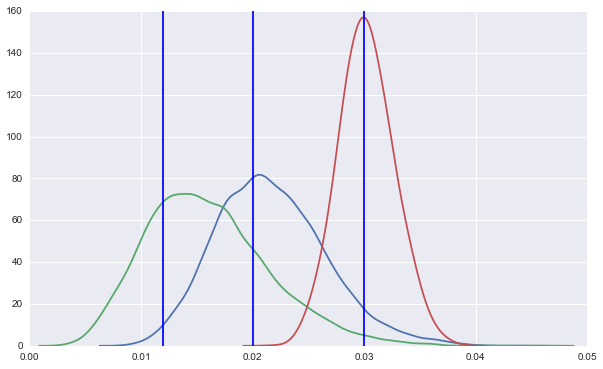
To run this, we just need to call step however many times we'd like. Here's a gif of training (each frame is a plot after 1000 events, and the vertical lines are the 'true CTRs'): Training with Argmax Draws

The height of each curve is a fair proxy for how much data populates it. Notice that as it becomes clear that the green distribution is the lowest performing, it basically doesn't get any higher. We stop showing this button. Initially, the blue curve looks like the winner, but again, as the red curve passes it, the height gains increasingly go to the winner.

Improvements over performance-agnostic bucketing

Another interesting comparison is: how different does this process go if you just randomly select a CTA rather than taking the CTA whose CTR distribution produced a winning draw? We can swap our draw_cta_index function for something like this:

def draw_cta_evenly():
    draws = UNIFORM.rvs(3)
    return draws.argmax()

Here's a comparison of our distributions after 6000 impressions between these models.
First, the 'winning beta' method:

We have good certainty about the winner, and the losers are only estimated (at this point) well enough to know they lost.
Then, the 'even draw' method:

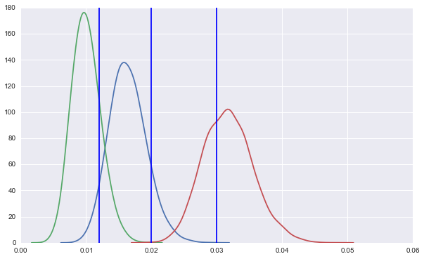
This is just one particular run, but clearly there's no favoring of higher-performance alternatives.
The winning beta method has significant impact in engagement: even in the first 1500 impressions, it produced, in this example, 20% more clicks. That number should only go up as the learning progresses and the impression-share of the winner increases.

Validating estimator properties

One nice thing about the "in the lab" example is we can see if the online model has the desired relationship to the ground truth. In particular, are our beta distributions higher variance when they're further from the truth? We can put add some logging to measure this.


ERROR_VAR_LOGS = []

def log_err_and_var():
    beta_mean_errs = np.abs(np.array(TRUE_CTR) - ctr_dist_means())
    beta_vars = np.array([x.var() for x in CTR_DISTS])
    for mean, var in zip(beta_mean_errs, beta_vars):
        ERROR_VAR_LOGS.append((mean, var))

It makes sense to call this periodically, since only one beta is updated each step; below are some results from collecting this data every 50 impressions:

error_df = pd.DataFrame(ERROR_VAR_LOGS, columns=('mean_error', 'dist_variance'))
error_df['dist_std'] = error_df['dist_variance'].apply(np.sqrt)
ax = error_df.plot(kind='scatter', x='mean_error', y='dist_std')

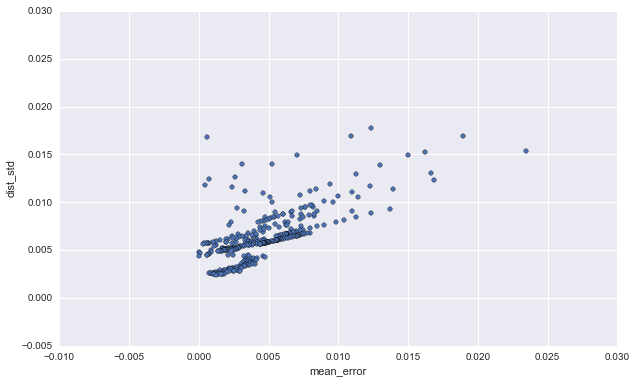
Happily, we see a positive relationship between error and distribution variance, so our tightening distributions are properly increasing confidence as they increase accuracy. The next part will outline how we can separate serving and selection processes and maintain render speed performance.